Verification

This page documents the verification tests that confirm every pretrained checkpoint produces correct TMRCA predictions. The simulated-data tests serve as a sanity check after installation and a reference for expected accuracy across model variants. The real-data test verifies the expected selective-sweep signal at the Rdl locus in Ag1000G mosquito data.

All verification scripts live in .verification/ at the repository root. Run them with:

python .verification/verify_all_models.py    # all seven checkpoints
python .verification/verify_input_types.py   # input-type consistency
python .verification/verify_rdl_5pops.py     # Rdl locus, 5 populations

Test protocol

Each model is verified by:

1. Simulating a tree sequence with msprime under constant \(N_e = 20{,}000\) (seed 42).

2. Running inference with 10 stochastic replicates on two pivot pairs.

3. Computing ground truth from the tree sequence’s exact genealogies.

4. Comparing predicted vs true log-TMRCA using MSE and Pearson correlation.

The w2000 models (broad, narrow, residual) are tested on 1 Mb sequences; the w200 models (broad_w200, w200_wmissing) on 100 kb. Adapter models use 5 diploid individuals (10 haploid samples).

In each figure below, the blue line is the mean prediction across 10 replicates, the blue shaded band shows \(\pm 2\sigma\), and the red line is the true TMRCA from the exact genealogy.

broad

The main 10-layer model trained on all scenarios. Tested on a 1 Mb constant \(N_e\) simulation with 50 haploid samples.

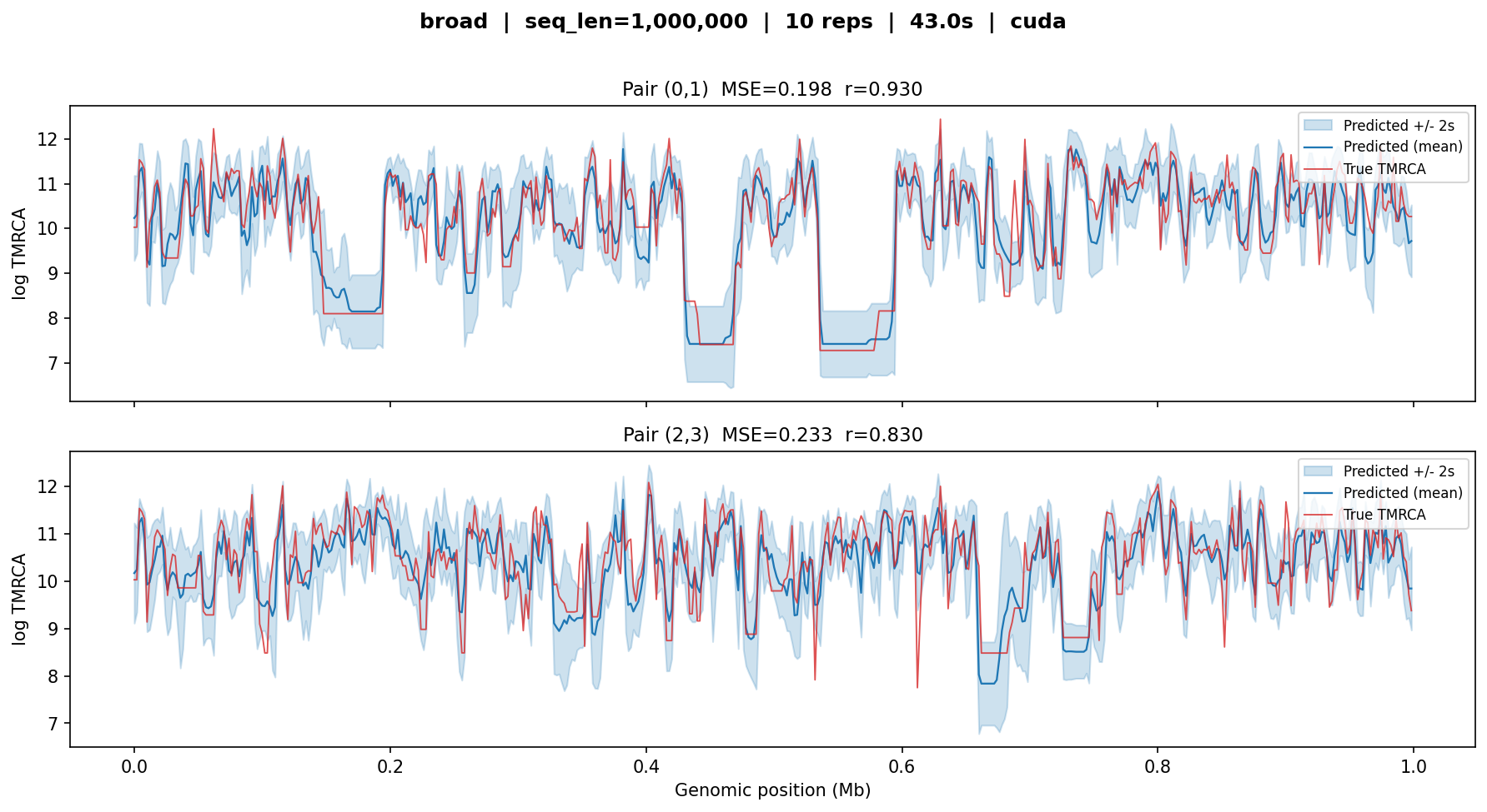
broad — MSE ≈ 0.2, r ≈ 0.83–0.93. The predicted curves closely track the true coalescent-time landscape across the full megabase, including sharp transitions at tree boundaries. Uncertainty bands are narrow relative to the signal.

narrow

The smaller 6-layer model trained only on constant \(N_e\) data. Despite having fewer layers and a simpler training set, it achieves comparable accuracy on this constant-\(N_e\) test case.

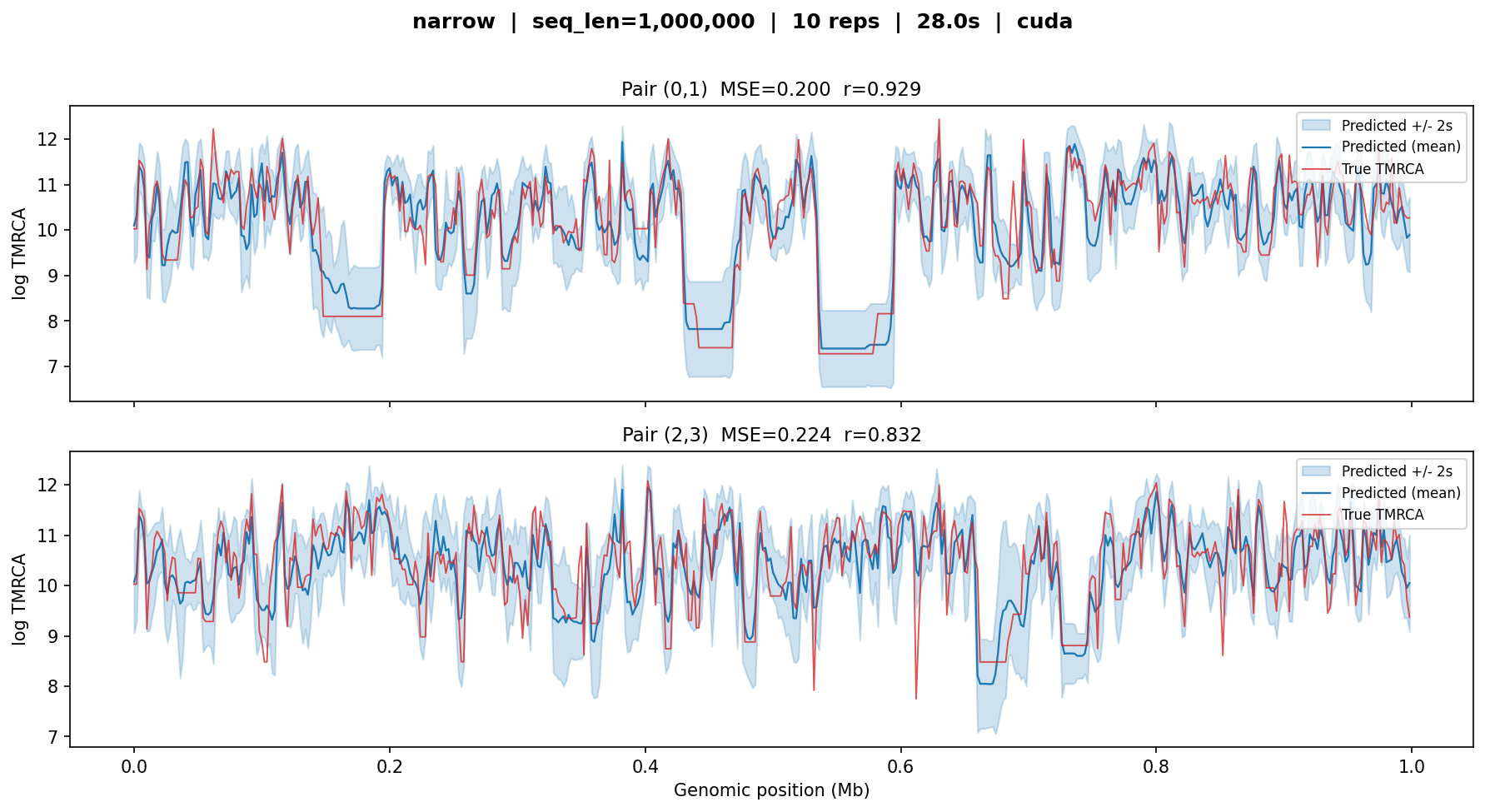
narrow — MSE ≈ 0.2, r ≈ 0.83–0.93. Nearly identical to broad on this constant-\(N_e\) simulation, as expected: the narrow model was trained specifically for this regime. Inference is faster (28 s vs 43 s) due to fewer layers.

residual

Predicts log-deviations from the population mean rather than absolute log-TMRCA. Higher MSE reflects the fact that this model targets a different objective: it sacrifices absolute-level accuracy for sharper resolution of relative TMRCA changes between adjacent windows.

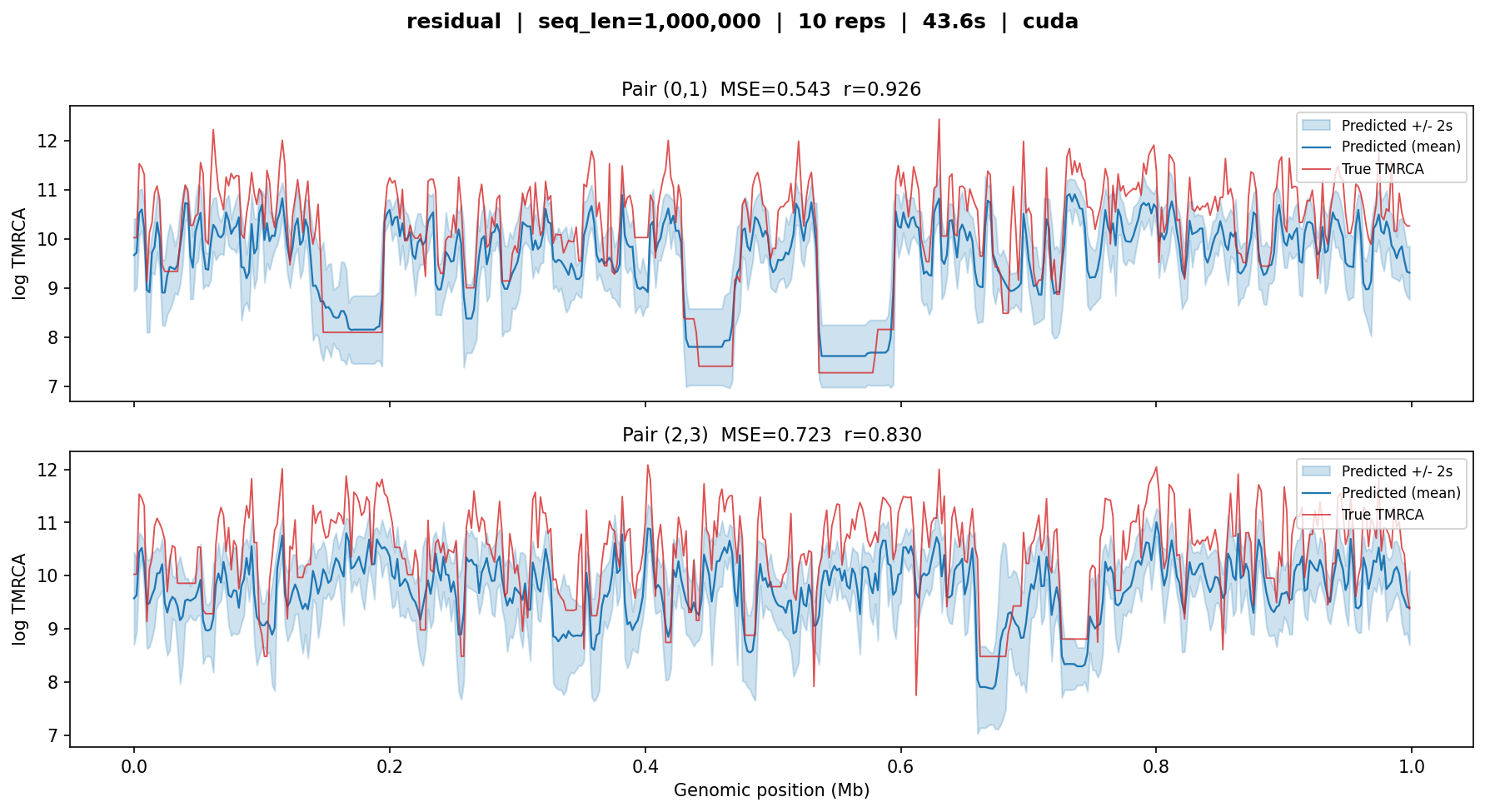
residual — MSE ≈ 0.5–0.7, r ≈ 0.83–0.93. The model tracks the shape of the coalescent-time profile well (high correlation) but shows a systematic upward shift in some regions, consistent with the residual parameterisation requiring a separate baseline estimate.

broad_w200

The broad model fine-tuned for 200 bp windows on large-\(N_e\) stdpopsim species. Tested on 100 kb (500 windows of 200 bp). The shorter sequence means fewer mutations per window and less information per prediction, so MSE is naturally higher than the w2000 models.

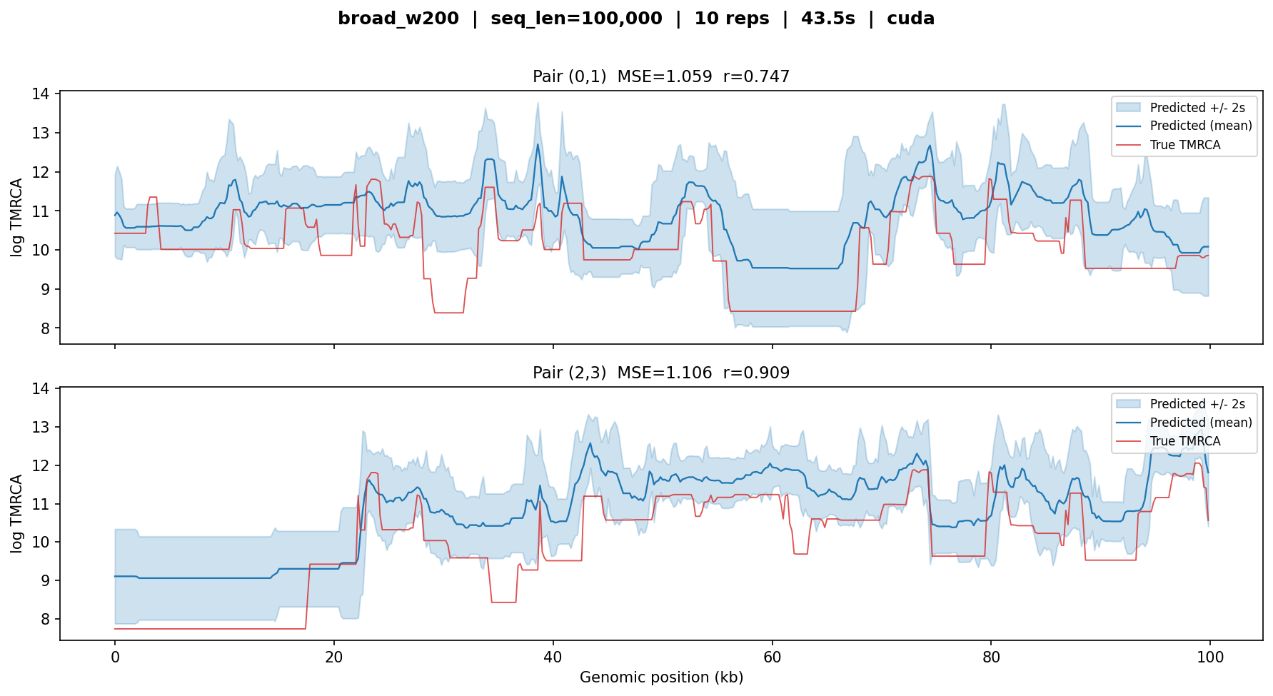
broad_w200 — MSE ≈ 1.0–1.1, r ≈ 0.75–0.91. Higher MSE compared to the w2000 models reflects the reduced mutational information per 200 bp window. Despite this, the model captures the major transitions in coalescent time and maintains strong correlation.

w200_wmissing

Fine-tuned from broad_w200 on data with encoded missingness (see Recipe: Fine-tuning for Missingness). This model expects a missingness_bitmask at inference time that encodes the per-window fraction of inaccessible sites.

Important

When running w200_wmissing on data with no missing sites, you must still pass an all-zeros bitmask:

missingness_bitmask = np.zeros(seq_len, dtype=bool)

Without this, the missingness channels in the source tensor are left unpopulated, and the model produces degraded predictions (MSE > 2, r < 0.65). With the correct bitmask, performance matches broad_w200.

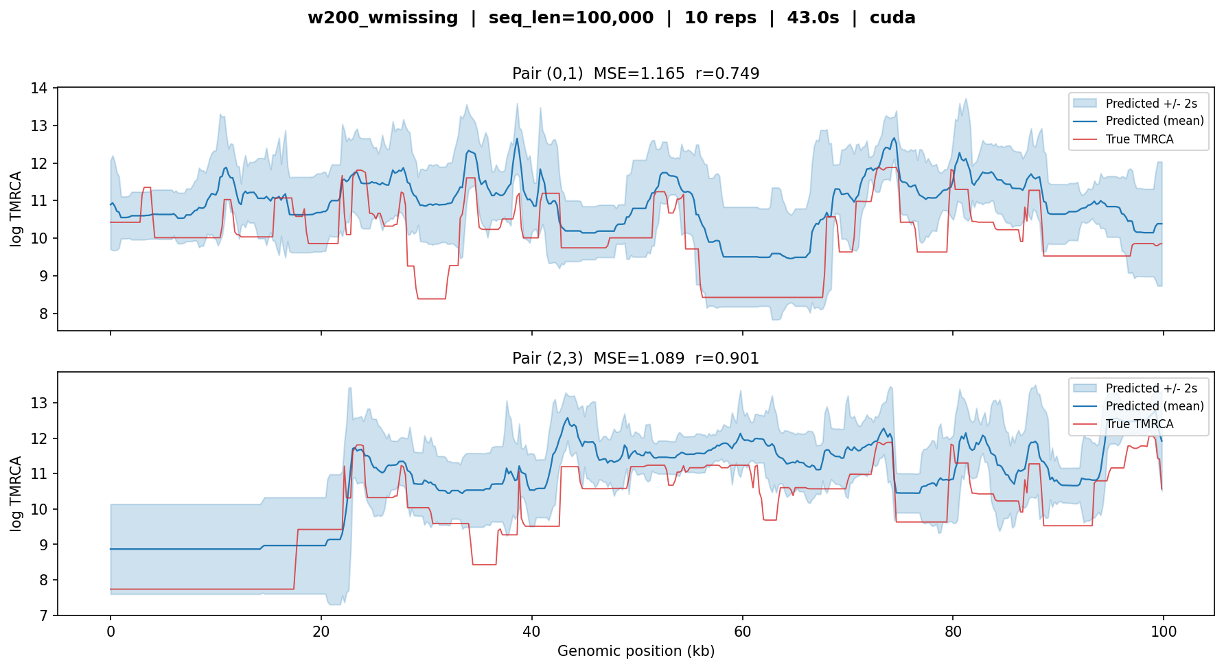
w200_wmissing — MSE ≈ 1.1–1.2, r ≈ 0.75–0.90. With the missingness bitmask set to all-accessible, the model performs comparably to its parent broad_w200.

broad+adapter

The sample-size adapter on top of a frozen broad backbone. Maps 10 haploid samples to the 50-sample feature space expected by the backbone. Tested on a 1 Mb simulation with 5 diploid individuals.

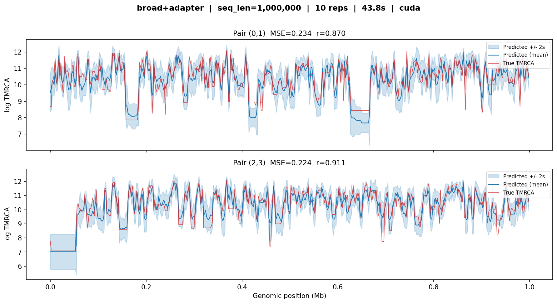
broad+adapter — MSE ≈ 0.2, r ≈ 0.87–0.91. The adapter produces results comparable to the full broad model despite working with only 10 haploid samples (5 diploids). Wider uncertainty bands reflect the reduced information from fewer samples.

w200_wmissing_adapter

Two-stage adapter combining sample-size transfer with missingness support. Built by resuming the broad+adapter weights on w200 + bitmask data. Tested on 100 kb with 5 diploid individuals.

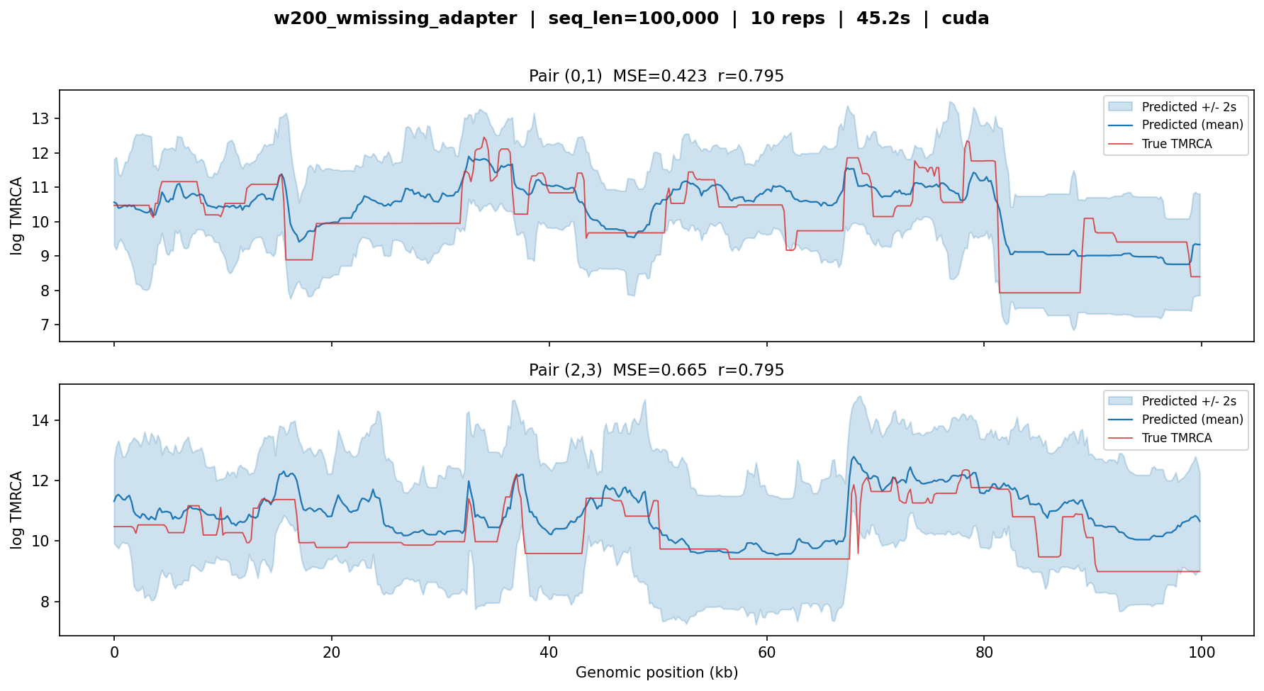
w200_wmissing_adapter — MSE ≈ 0.4–0.7, r ≈ 0.80. Combines the challenges of small sample size (10 haplotypes), fine window resolution (200 bp), and missingness encoding. The higher MSE and wider uncertainty bands reflect these compounding difficulties. Correlation remains good, indicating the model captures the shape of the coalescent-time landscape.

Rdl locus — Ag1000G real-data verification

In addition to the simulated-data tests above, we verify the w200_wmissing and w200_wmissing_adapter models on real data from the Ag1000G Anopheles gambiae dataset. The test runs cxt inference from scratch on the Rdl insecticide-resistance locus (25.1–25.6 Mb on chr2L) across five African populations: Mali, Burkina Faso, Cameroon, Uganda, and Ghana.

The expected signal is a sharp TMRCA trough at the Rdl gene (25.36–25.43 Mb), consistent with a selective sweep driven by dieldrin resistance. The four larger populations (25 diploid individuals each) use the w200_wmissing model; Ghana (5 diploid individuals) uses the w200_wmissing_adapter model. Each population is inferred using 25 pairs from inversion-heterozygote (2La = 1) individuals.

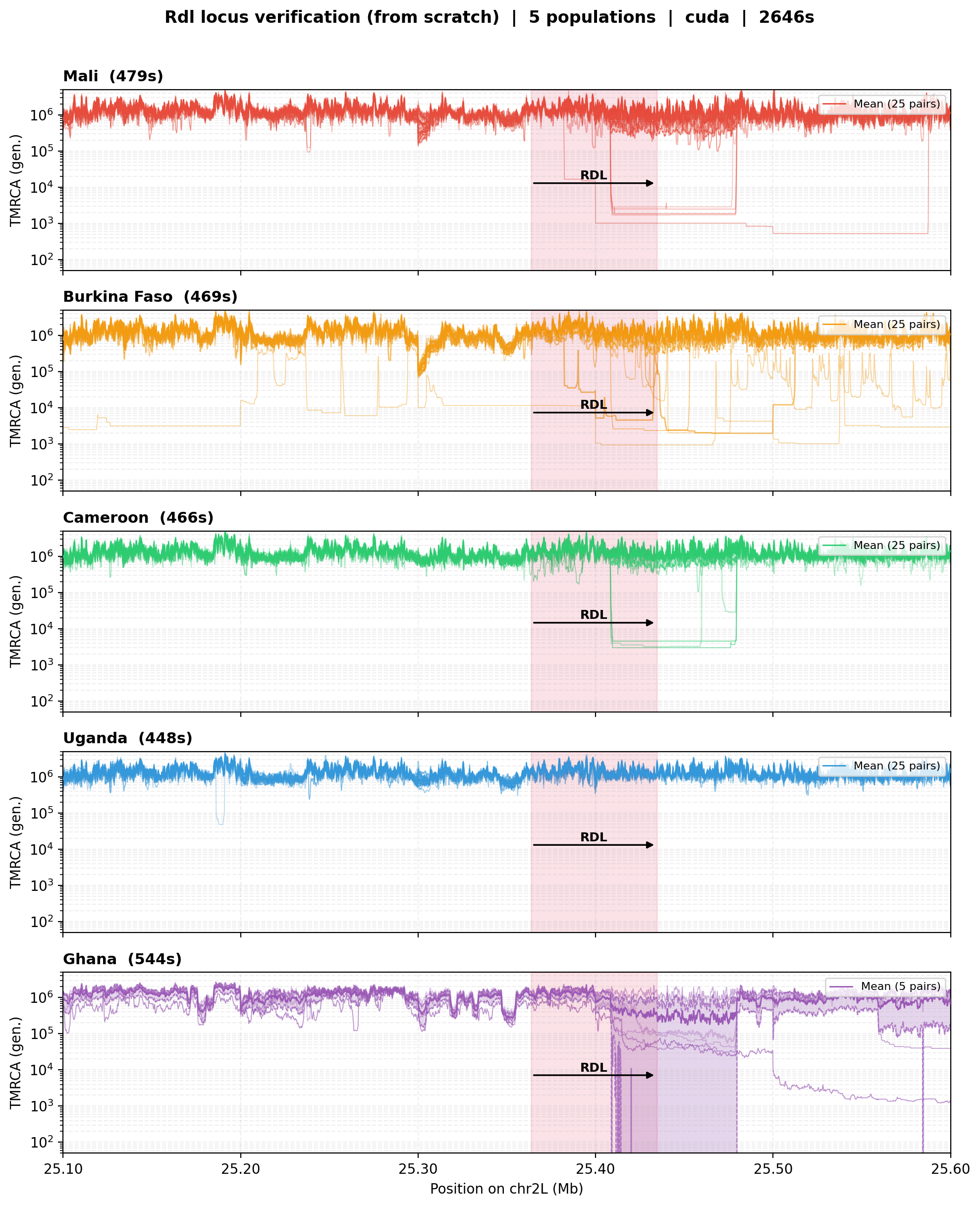
Rdl locus verification. Per-pair TMRCA traces (coloured lines) and mean ± SD band across the Rdl region for all five Ag1000G populations. The red shaded region marks the Rdl gene. Mali and Burkina Faso show the strongest sweep signatures, with multiple pairs dropping to \(\sim 10^{2}\)–\(10^{3}\) generations at the locus. Cameroon and Ghana show clear sweeps in a subset of pairs. Uganda shows a more subtle signal, consistent with lower insecticide pressure in East Africa.

python .verification/verify_rdl_5pops.py

This test requires the Ag1000G chr2L tree sequence and accessibility mask (see Mosquito: 2L Inversion and RDL Sweep for data setup). Population tree sequences are cached in .verification/cache_rdl/ after the first run. Inference runs on just the five 100 kb blocks covering the Rdl region, taking approximately 8 minutes per population on a single GPU.

Input-type consistency

cxt accepts three input types: tree sequences, genotype matrices, and VCF files. This test verifies that all three produce identical results by simulating a 1 Mb tree sequence, exporting it to both a genotype matrix and a VCF, and running inference through each path with the broad model.

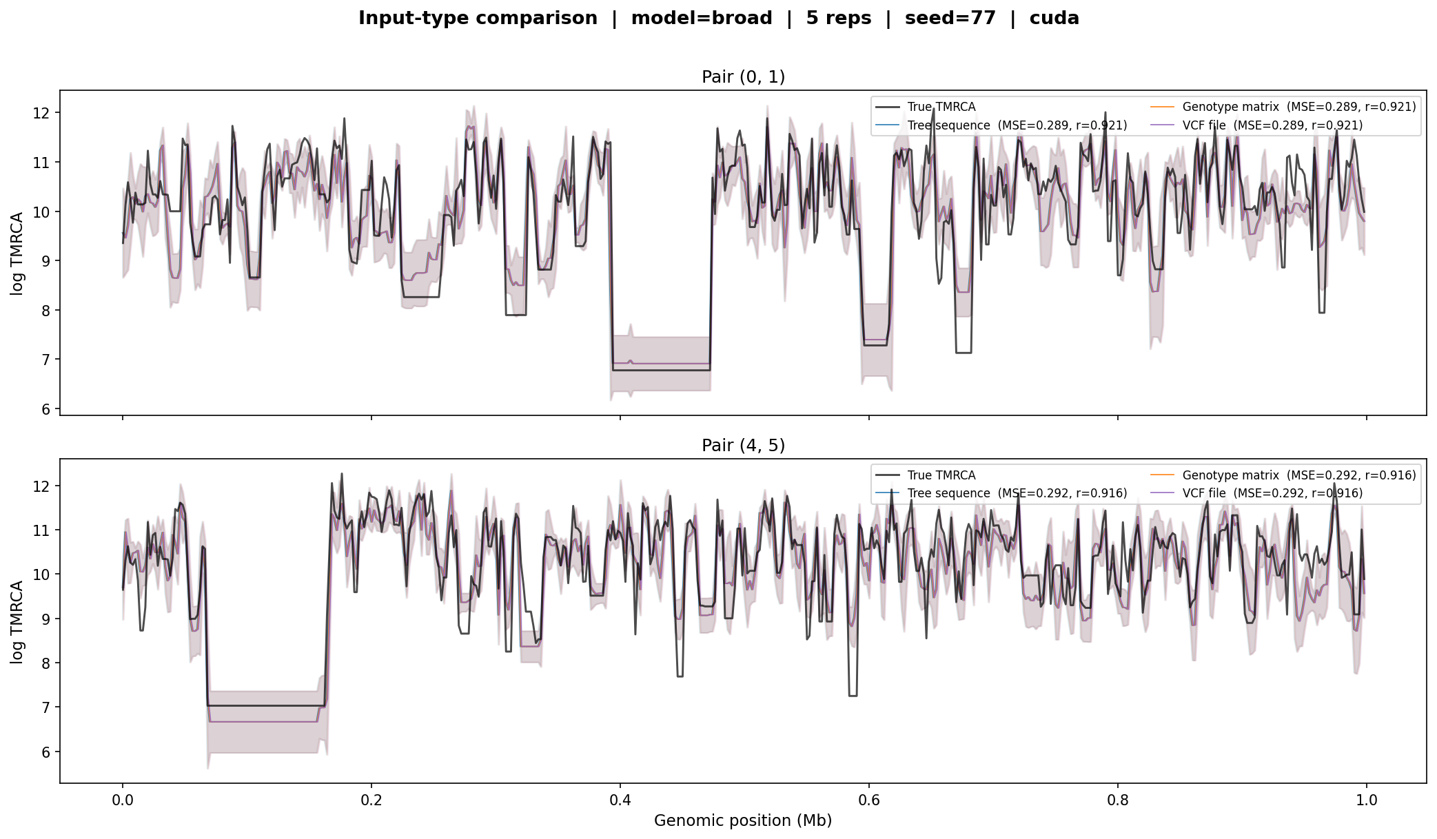
Input-type comparison. The tree-sequence, genotype-matrix, and VCF input paths produce indistinguishable TMRCA predictions (identical MSE and correlation for each pair). All three curves overlap completely.

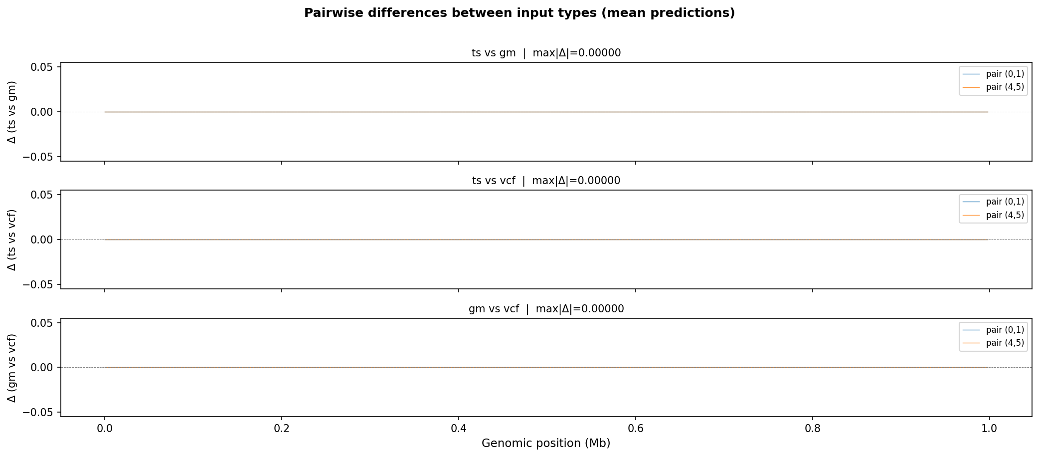
Pairwise differences between input types. The maximum absolute difference between any two input paths is zero across the entire genome, confirming that the three code paths are numerically equivalent.

Summary table

Model	Seq length	Samples	MSE	r	Time (s)
broad	1 Mb	50	0.2	0.83–0.93	43
narrow	1 Mb	50	0.2	0.83–0.93	28
residual	1 Mb	50	0.5–0.7	0.83–0.93	44
broad_w200	100 kb	50	1.0–1.1	0.75–0.91	44
w200_wmissing	100 kb	50	1.1–1.2	0.75–0.90	43
broad+adapter	1 Mb	10	0.2	0.87–0.91	44
w200_wmissing_adapter	100 kb	10	0.4–0.7	0.80	45

Running the verification

# Verify all seven checkpoints (downloads ~700 MB on first run)
python .verification/verify_all_models.py

# Verify input-type consistency (tree sequence vs genotype matrix vs VCF)
python .verification/verify_input_types.py

# Verify Rdl locus on Ag1000G data (requires tree sequence + accessibility mask)
python .verification/verify_rdl_5pops.py

Checkpoints are cached in .verification/checkpoints/ and reused on subsequent runs. Set the CXT_CHECKPOINT_CACHE environment variable to redirect the cache. The Rdl verification uses checkpoints from the BASE_DIR path (default /sietch_colab/data_share/cxt_scratch).