Human 1000 Genomes: LCT and HLA
This example applies cxt to GBR samples from the 1000 Genomes Project to decode chromosome-scale TMRCA landscapes and zoom into the LCT locus (chromosome 2) and HLA region (chromosome 6).
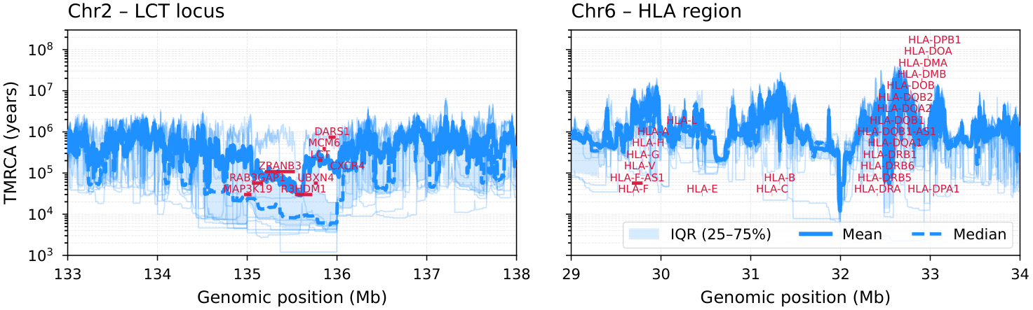
Figure 6 (top). Inference of coalescent times from 25 focal pairs of British individuals from the 1000 Genomes Project. Chromosome-wide TMRCA landscapes for chromosomes 2 (left) and 6 (right).
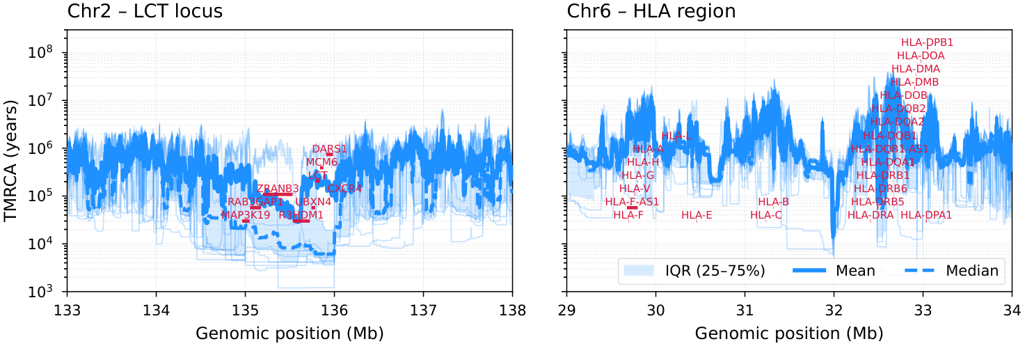
Figure 6 (bottom). Zoomed view of the LCT region on chromosome 2 (left) and the HLA region on chromosome 6 (right). Each pivot pair has been inferred 15 times to get reliable mean, median, and variance estimates. Light blue lines show the respective inferences of the 25 pairs; the IQR (25–75%) band, mean, and median are overlaid with gene annotations.
Pipeline overview
Load tsinfer-based tree sequences for chr2p/chr2q and chr6p/chr6q.
Run
cxt.translate()in 1 Mb blocks on 25 pivot pairs.Apply a post-hoc stochastic diversity-based bias correction.
Stitch p and q arms into whole-chromosome TMRCA tracks.
Plot chromosome-wide curves and zoom into LCT and HLA with gene annotations.
Note
Unlike the mosquito analysis, we do not use a missingness-aware model variant here. Instead, a post-hoc stochastic diversity bias correction accounts for the moderate missingness in these human regions.
Model and devices
import os
import numpy as np
import torch
import tszip
import cxt

devices = [f"cuda:{i}" for i in range(torch.cuda.device_count())]
model = cxt.load_model("broad", device="cpu")

cache_dir = "./cache"
os.makedirs(cache_dir, exist_ok=True)
Loading GBR tree sequences
We load precomputed tsinfer-based trees for four chromosome arms, simplify to 50 haploid samples, and cache locally:
TSZ_DIR = "/path/to/hg1kg/tsinfer-trees"

arms = {}
for arm_name in ["chr2p", "chr2q", "chr6p", "chr6q"]:
    tsz_cache = os.path.join(cache_dir, f"gbr_{arm_name}.tsz")
    if os.path.exists(tsz_cache):
        arms[arm_name] = tszip.load(tsz_cache)
    else:
        ts = tszip.load(os.path.join(TSZ_DIR, f"{arm_name}.tsz"))
        ts = ts.simplify(samples=np.arange(50))
        tszip.compress(ts, tsz_cache)
        arms[arm_name] = ts

    print(f"{arm_name}: {arms[arm_name].num_samples} samples, "
          f"{arms[arm_name].sequence_length:.0f} bp")
Inference on 1 Mb blocks
We tile each arm into 1 Mb blocks and use 25 consecutive pivot pairs:
pivot_pairs = [(i, i + 1) for i in range(0, 50, 2)]

def infer_arm(ts, name):
    cache_path = os.path.join(cache_dir, f"gbr_{name}.npz")
    if os.path.exists(cache_path):
        data = np.load(cache_path)
        return data["tmrca"], data["index_map"]

    num_blocks = int(ts.sequence_length // 1e6)
    blocks = [(int(i * 1e6), int((i + 1) * 1e6)) for i in range(num_blocks)]

    tmrca, index_map = cxt.translate(
        ts, model,
        pivot_pairs=pivot_pairs,
        blocks=blocks,
        B_per_device=128, B=128,
        devices=devices,
        build_workers=32,
    )
    np.savez_compressed(cache_path, tmrca=tmrca, index_map=index_map)
    return tmrca, index_map

results = {}
for arm_name, ts in arms.items():
    results[arm_name] = infer_arm(ts, arm_name)
Post-hoc diversity correction
We estimate per-window missingness from bcftools masks and apply a stochastic diversity-based correction per block:
from cxt.correction import stochastic_diversity_bias_correction

mutation_rate = 1.29e-8

def correct_arm(tmrca, index_map, ts, availability, name):
    cache_path = os.path.join(cache_dir, f"genome_{name}.npz")
    if os.path.exists(cache_path):
        return np.load(cache_path)["genome"]

    num_blocks = int(ts.sequence_length // 1e6)
    blocks = [(int(i * 1e6), int((i + 1) * 1e6)) for i in range(num_blocks)]

    corrected_blocks = []
    for b_idx in range(num_blocks):
        mask = index_map[:, 0] == b_idx
        block = blocks[b_idx]
        avail = availability[b_idx] / 100 if availability is not None else 1.0

        try:
            ts_block = ts.keep_intervals([block], simplify=True)
            rng = np.random.default_rng(20_000_001 + b_idx)
            out = stochastic_diversity_bias_correction(
                tree_sequence=ts_block,
                mutation_rate=mutation_rate / max(avail, 0.01),
                predictions=tmrca[:, mask],
                pivot_pairs=np.array(pivot_pairs),
                rng=rng,
            )
            corrected_blocks.append(out.mean(0))
        except Exception:
            corrected_blocks.append(np.zeros([25, 500]))

    genome = np.stack(corrected_blocks).transpose(1, 0, 2).reshape(25, -1)
    np.savez_compressed(cache_path, genome=genome)
    return genome
Stitching chromosome-wide tracks
genome_chr2 = (
    correct_arm(*results["chr2p"], arms["chr2p"], chr2_available, "chr2p")
    + correct_arm(*results["chr2q"], arms["chr2q"], chr2_available, "chr2q")
)
genome_chr6 = (
    correct_arm(*results["chr6p"], arms["chr6p"], chr6_available, "chr6p")
    + correct_arm(*results["chr6q"], arms["chr6q"], chr6_available, "chr6q")
)
Chromosome-wide plot
import matplotlib.pyplot as plt

generation_time = 28
BIN_BP = 2000

lct_start, lct_end = 135_300_000, 136_400_000
hla_start, hla_end = 29_600_000, 33_300_000

fig, axes = plt.subplots(1, 2, figsize=(12, 3), sharex=False, sharey=True)

for ax, genome, label in [
    (axes[0], genome_chr2, "Chromosome 2"),
    (axes[1], genome_chr6, "Chromosome 6"),
]:
    x = np.arange(genome.shape[1]) * BIN_BP
    y = np.exp(genome.mean(0)) * generation_time
    ax.plot(x, y, linewidth=0.8, color="dodgerblue", alpha=0.9)
    ax.set_yscale("log")
    ax.set_title(label, loc="left", fontsize=12)
    ax.grid(alpha=0.3, which="both", linestyle="--")

axes[0].axvspan(lct_start, lct_end, color="crimson", alpha=0.3, label="LCT")
axes[1].axvspan(hla_start, hla_end, color="crimson", alpha=0.3, label="HLA")
axes[0].text(lct_start, 3e6, "LCT", color="crimson", fontsize=10, va="bottom")
axes[1].text(hla_start, 3e6, "HLA", color="crimson", fontsize=10, va="bottom")

fig.text(0.5, 0.03, "Position (bp)", ha="center", fontsize=12)
fig.text(0.04, 0.5, "Mean TMRCA (years)", va="center",
         rotation="vertical", fontsize=12)

plt.tight_layout(rect=[0.05, 0.05, 1, 0.95])
plt.ylim(1e3, 1e7)
fig.savefig("figure6_human_1kg.png", dpi=300, bbox_inches="tight")
Zoomed panels with gene annotations
The zoomed LCT and HLA panels overlay individual replicate traces, IQR bands, and gene annotations. Key genes at each locus:
LCT region (chr2, 133–138 Mb): LCT, MCM6, DARS1, R3HDM1, ZRANB3, UBXN4, RAB3GAP1, CXCR4
HLA region (chr6, 29–34 Mb): HLA-A, HLA-B, HLA-C, HLA-DRB1, HLA-DQA1, HLA-DQB1, HLA-DPA1, HLA-DPB1
The plotting code is available in figures/main/fig6_human_1kg.py.
The LCT region shows a sharp reduction in TMRCA consistent with the well-documented signature of recent positive selection on lactase persistence in European populations. The HLA region displays elevated and highly variable TMRCA, reflecting ancient balancing selection maintaining MHC diversity.