Demography Inference and Coalescence Rates

Estimating pairwise coalescence rates provides a direct window into changes in effective population size through time. This page demonstrates how to convert cxt’s TMRCA predictions into coalescence-rate curves and compares them against Singer+Polegon and SMC++ on three species: H. sapiens (Zigzag_1S14), A. thaliana (SouthMiddleAtlas_1D17), and B. taurus (HolsteinFries_1M13), all from stdpopsim.

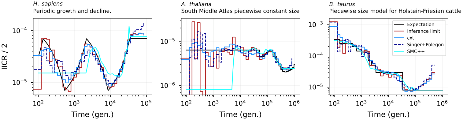
Figure 5. Inverse-instantaneous coalescence rate (IICR) calculation for the piecewise-constant demography of (A) H. sapiens, (B) A. thaliana, and (C) B. taurus. The inference of pairwise-coalescence events leads to the implicit inference of demography estimates through the marginal coalescence distribution assuming coalescence occurs as a Poisson process. For each scenario 10 Mb and 25 diploid samples have been used to achieve resolution throughout the specified time windows.

Setup and imports

import os
import numpy as np
import tskit
import torch
import stdpopsim
import matplotlib.pyplot as plt
from tqdm import tqdm

import cxt
from cxt.utils import coalescence_rates
from cxt.preprocess import interpolate_tmrcas

cache_dir = "./cache"
os.makedirs(cache_dir, exist_ok=True)

devices = [f"cuda:{i}" for i in range(torch.cuda.device_count())]
model = cxt.load_model("broad", device="cpu")

Simulating Zigzag_1S14 with stdpopsim

We simulate 25 diploid individuals under the human Zigzag_1S14 demography for 10 Mb of chromosome 1:

num_pairs = 25
window_size = 2e3
seed = int(10e6)
sequence_length = 10e6

species = stdpopsim.get_species("HomSap")
demogr = species.get_demographic_model("Zigzag_1S14")
contig = species.get_contig("chr1", right=sequence_length)

population_name = demogr.populations[0].name
sample = {population_name: num_pairs}
engine = stdpopsim.get_engine("msprime")

ts_path = os.path.join(cache_dir, "homsap.ts")
if not os.path.exists(ts_path):
    ts = engine.simulate(
        contig=contig, samples=sample,
        demographic_model=demogr, seed=seed,
    ).trim()
    ts.dump(ts_path)
else:
    ts = tskit.load(ts_path)

Computing true TMRCAs

We compute discretized true TMRCAs for all pairwise combinations among the 25 individuals:

true_path = os.path.join(cache_dir, "homsap_true_tmrcas.npy")
if os.path.exists(true_path):
    true_tmrcas = np.load(true_path)
else:
    pivot_ids = []
    true_tmrcas = []
    for i in tqdm(range(num_pairs)):
        for j in range(i + 1, num_pairs):
            pivot_ids.append((i, j))
            tmrca_ij = interpolate_tmrcas(
                ts, window_size=int(window_size),
                sample_a=i, sample_b=j,
            )
            true_tmrcas.append(tmrca_ij)
    true_tmrcas = np.array(true_tmrcas)
    np.save(true_path, true_tmrcas)

Running cxt

We analyze the 10 Mb region in 10 non-overlapping 1 Mb blocks:

blocks = [(int(x), int(x + 1e6))
          for x in np.linspace(0, 9e6, 10)]

pivot_pairs = [(i, j)
               for i in range(num_pairs)
               for j in range(i + 1, num_pairs)]

tmrca_path = os.path.join(cache_dir, "tmrca_homsap.npz")
if os.path.exists(tmrca_path):
    data = np.load(tmrca_path)
    tmrca, index_map = data["tmrca"], data["index_map"]
else:
    tmrca, index_map = cxt.translate(
        ts, model,
        pivot_pairs=pivot_pairs,
        blocks=blocks,
        B_per_device=128, B=128,
        devices=devices,
        build_workers=32,
        mutation_rate=1.29e-8,
    )
    np.savez_compressed(tmrca_path, tmrca=tmrca, index_map=index_map)

Estimating coalescence rates

We convert windowed TMRCAs into coalescence-rate curves using cxt.utils.coalescence_rates() and compare them to the theoretical trajectory from the demographic model:

num_time_windows = 40
max_log_time = np.floor(np.log10(ts.max_time))

time_windows = np.logspace(2, max_log_time, num_time_windows + 1)
time_windows[0] = 0.0

fine_time_grid = np.logspace(2, max_log_time, 1000)
coalrate_ck, _ = demogr.model.debug().coalescence_rate_trajectory(
    lineages={population_name: 2}, steps=fine_time_grid,
)

tmrca_flat = np.exp(tmrca.flatten())
true_tmrcas_flat = true_tmrcas.flatten()

yhat_coalrate = coalescence_rates(tmrca_flat, time_windows)
ytrue_coalrate = coalescence_rates(true_tmrcas_flat, time_windows)

Plotting coalescence rates

fig, ax = plt.subplots(figsize=(6, 4))

ax.step(time_windows[:-1], yhat_coalrate, where="post",
        label=r"$\mathbf{cxt}$", color="dodgerblue")
ax.step(time_windows[:-1], ytrue_coalrate, where="post",
        label="inference limit (discrete)", color="firebrick")
ax.plot(fine_time_grid, coalrate_ck, "-", color="black",
        label="demographic expectation")

ax.set_xscale("log")
ax.set_yscale("log")
ax.set_xlabel("Time (generations)")
ax.set_ylabel("Coalescence rate")
ax.grid(True, which="both", alpha=0.3)
ax.set_title(r"$\it{H.\;sapiens}$ Zigzag_1S14", loc="left")
ax.legend()
fig.tight_layout()
fig.savefig("figure5_demography.png", dpi=300)

stdpopsim benchmark figures

The paper includes additional benchmarks on the full stdpopsim species catalog. These panels show KDE distributions of TMRCA predictions compared to the inference limit across multiple species.

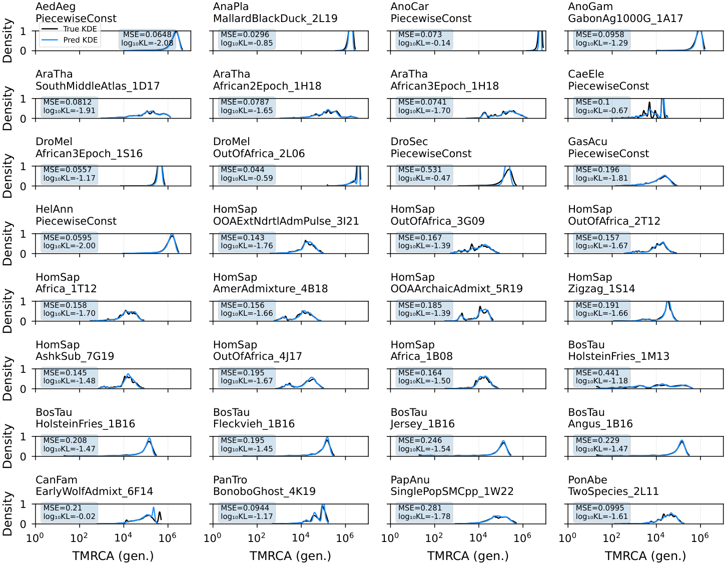
Figure 3. Evaluation of marginal coalescence distribution inference (blue line) against the true distribution (black line), probing the model’s capacity to distinguish among many scenarios based on context alone. The broad model’s ability to infer a stdpopsim v0.2 coalescence distribution is tested, which includes diverse mutation and recombination rates, as well as demographic scenarios. All results shown are from new simulations, not included in the original training dataset. No genetic map was used for the inference shown here.

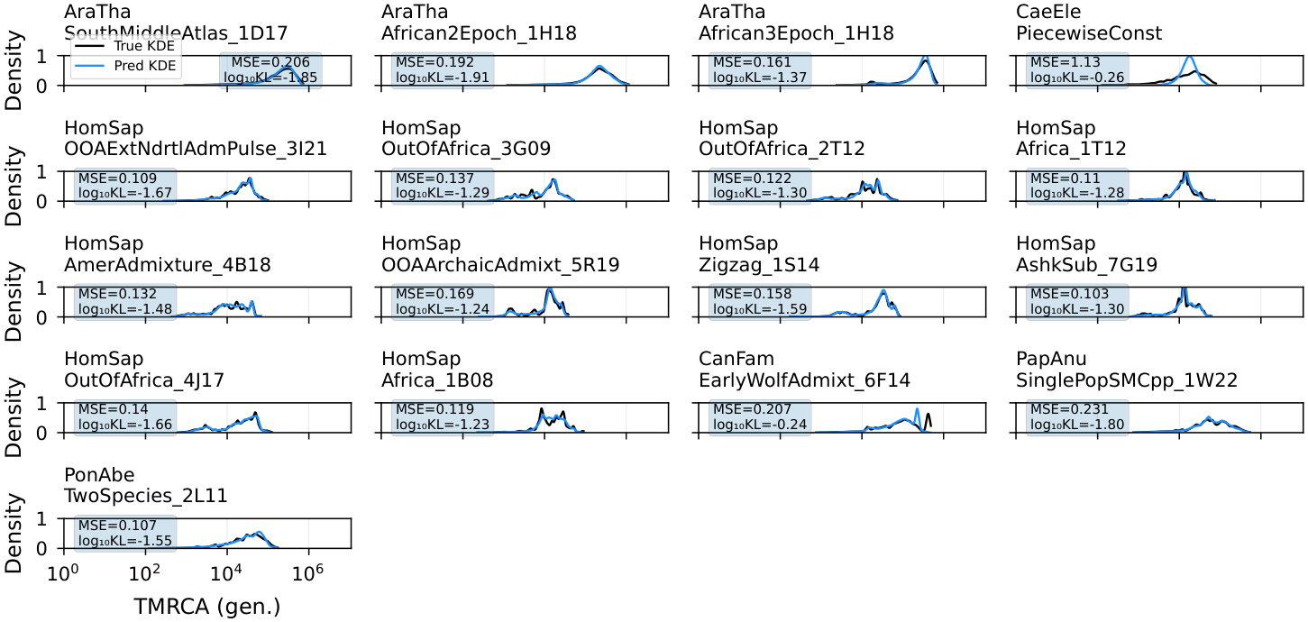
Figure 3 (genetic maps). Same evaluation with an underlying genetic map. The model itself was trained with and without genetic maps.

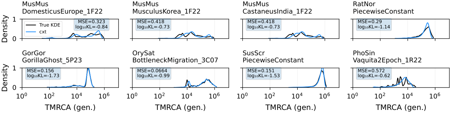
Figure 4. Out-of-sample evaluation of the broad model on stdpopsim v0.3. Each panel shows inferred marginal coalescence distributions (dashed) against true distributions (shaded). Data were simulated from the novel species and demographic histories added in stdpopsim v0.3. All results are from simulations previously unseen during training (top row: cxt; middle row: Singer+Polegon; bottom row: SMC++).