Quick Start

This page demonstrates the core cxt workflow in under 20 lines of code: simulate a tree sequence, run inference, and compare inferred versus true coalescent times.

Minimal example

import cxt
import msprime
import numpy as np

# 1. Simulate a 1 Mb tree sequence
ts = msprime.sim_ancestry(
    25, population_size=2e4, sequence_length=1e6,
    recombination_rate=1.28e-8, random_seed=42,
)
ts = msprime.mutate(ts, rate=1.29e-8, random_seed=42)

# 2. Load a pretrained model
model = cxt.load_model("broad", device="cuda")

# 3. Infer TMRCA for selected haplotype pairs
tmrca, index_map = cxt.translate(
    ts, model,
    blocks=[(0, 1_000_000)],
    pivot_pairs=[(0, 1), (2, 3), (4, 5)],
    devices=["cuda:0"],
    n_reps=15,
    mutation_rate=1.29e-8,
)

# tmrca shape: (n_items, n_reps, n_windows) -- log-TMRCA values
print(f"Inferred TMRCA shape: {tmrca.shape}")

Benchmark: constant \(N_e\)

The following example reproduces the narrow-model constant-\(N_e\) benchmark scatter plot from the paper. It compares inferred TMRCAs against the true values from the simulated tree sequence.

import os
import numpy as np
from concurrent.futures import ProcessPoolExecutor

import cxt
from cxt.utils import simulate_parameterized_tree_sequence
from cxt.preprocess import interpolate_tmrcas

# Simulate
ts = simulate_parameterized_tree_sequence(seed=103370001)

# Load model
model = cxt.load_model("narrow", device="cuda")

# All pairwise combinations among 50 haploid samples
pivot_pairs = [(i, j) for i in range(50) for j in range(i + 1, 50)]

# Infer
yhat_tmrca, index_map = cxt.translate(
    ts, model,
    pivot_pairs=pivot_pairs,
    blocks=[(0, 1_000_000)],
    devices=["cuda:0", "cuda:1", "cuda:2"],
    B=256,
    build_workers=8,
    mutation_rate=1.29e-8,
)

# Compute true TMRCAs
def _true(args):
    ts, a, b = args
    return interpolate_tmrcas(
        ts, window_size=2000, sample_a=a, sample_b=b,
    )

with ProcessPoolExecutor(max_workers=24) as ex:
    ytrues = list(ex.map(_true, [(ts, a, b) for a, b in pivot_pairs]))

yhats = [np.exp(yhat_tmrca).mean(0)[i] for i in range(len(pivot_pairs))]

# Scatter plot
from cxt.utils import plot_inference_scatter

plot_inference_scatter(
    np.array(yhats).flatten(),
    np.array(ytrues).flatten(),
    "cxt_constant.png",
    tool=r"$\mathbf{cxt}$-narrow: Constant $N_e$",
)

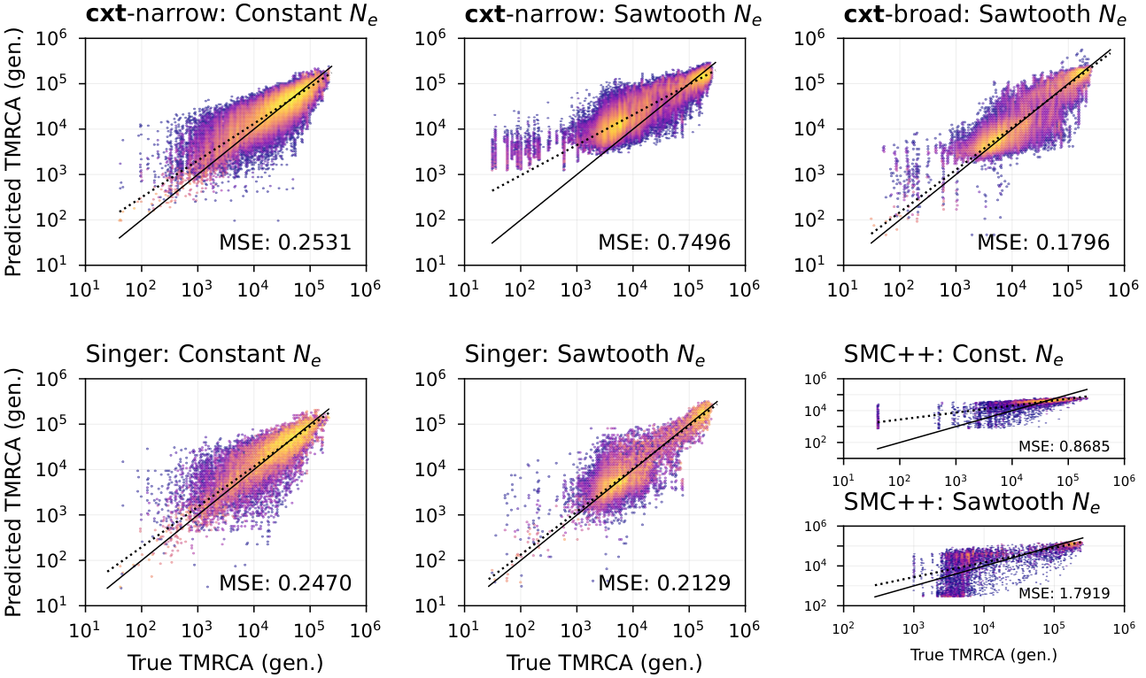
Figure 2. True versus predicted coalescence times for three inference approaches across two demographic scenarios: a constant population size and a fluctuating “sawtooth” demography. Top row: cxt-narrow evaluated on the constant-size scenario (left) and on the sawtooth scenario (middle), followed by cxt-broad evaluated on the sawtooth scenario (right). Bottom row: Singer+Polegon evaluated on the constant-size (left) and sawtooth (middle) scenarios, followed by SMC++ on the constant-size and sawtooth scenarios. MSE values are reported within each panel.

Input formats

cxt accepts three input types via the unified cxt.translate() interface:

Tree sequence (default):

tmrca, index_map = cxt.translate(ts, model, ...)

VCF file:

tmrca, index_map = cxt.translate("path/to/file.vcf", model, ...)

Genotype matrix (gm, positions) tuple:

import numpy as np
gm = np.load("genotypes.npy")     # (n_haplotypes, n_sites)
pos = np.load("positions.npy")    # (n_sites,) in bp

tmrca, index_map = cxt.translate(
    (gm, pos), model, ...
)

Note

Two usage patterns arise naturally depending on how blocks and pivot pairs are specified:

• Targeted: many pivot pairs on few narrow blocks – concentrates inference on specific loci.

• Long-range: few pivot pairs across many contiguous blocks – enables chromosome-scale TMRCA decoding.