Mosquito: 2L Inversion and RDL Sweep

This example applies cxt to Anopheles gambiae (Ag1000G) data on chromosome 2L to visualize coalescent-time patterns across the 2La inversion and the RDL insecticide-resistance locus.

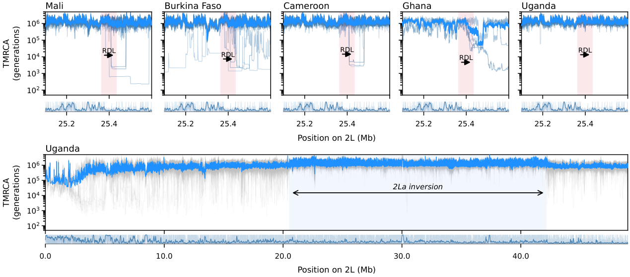
Figure 7. Inference of coalescent-time landscapes in the Ag1000G A. gambiae dataset across five African populations using cxt. In the upper panel, we analyze the Rdl region for Burkina Faso, Mali, Cameroon, Ghana, and Uganda. For these countries, we infer coalescent times for 25 focal haplotype pairs per population; for Ghana, we analyze five diploid individuals. Light-blue curves indicate per-pair coalescent-time trajectories inferred by cxt, with the mean trend shown in darker blue. The lower panel shows genome-wide coalescent-time landscapes across the entirety of chromosome 2L for Uganda samples. Missing data density is shown beneath both the regional and genome-wide panels as a genome browser track.

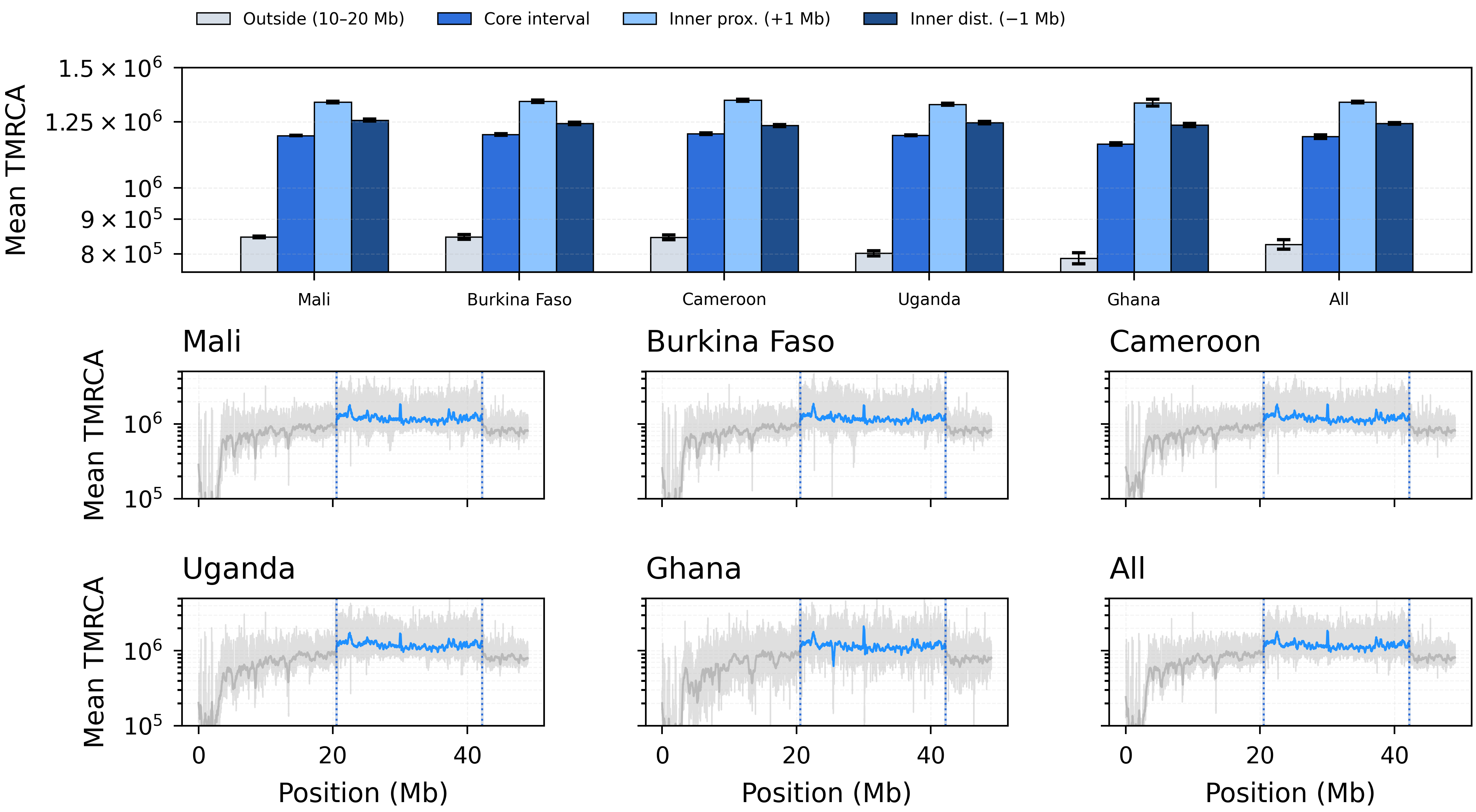
Figure 8. Coalescent-time structure across the In(2L)a inversion on chr2L. Top: mean TMRCA summaries for an outside background region (10–20 Mb), the full inversion core interval, and two interior 0.5 Mb windows positioned 1 Mb inside each breakpoint (mean \(\pm\) s.e.m. across replicate trajectories; “All” aggregates populations). Bottom: genome-wide mean TMRCA curves shown per population and pooled (“All”), with vertical guides marking inversion boundaries, breakpoint-adjacent windows, and the interior sampling windows used for summary statistics. Note that Ghana uses fewer haplotypes (n = 10) and a sample-size adapter, yielding higher variance and slightly elevated breakpoint-region estimates relative to its genomic baseline.

Pipeline overview

1. Load and subset Ag1000G 2L tree sequences per population and inversion genotype (2La heterozygotes).

2. Load the accessibility bitmask and derive missingness tracks.

3. Run cxt.translate() with the missingness-aware model variant (w200_wmissing).

4. For Ghana (fewer available individuals), use the w200_wmissing_adapter model with 10-sample input.

5. Aggregate TMRCAs per genome and per population.

6. Plot the RDL zoom panel and the genome-wide inversion panel.

Model and data setup

import os
import json
import numpy as np
import torch
import tskit
import cxt

cache_dir = "./cache"
os.makedirs(cache_dir, exist_ok=True)

data_path = "/path/to/Ag1000G/gamb.2L.gff.dated.ne.trees"
accessible_path = "/path/to/Ag1000G/agp3.is_accessible.txt.npz"

devices = [f"cuda:{i}" for i in range(torch.cuda.device_count())]

model = cxt.load_model("w200_wmissing", device="cpu")
adapter_model = cxt.load_model("w200_wmissing_adapter", device="cpu")

Loading and subsetting populations

We subset the full 2L tree sequence to 2La heterozygous individuals from each population:

POPULATIONS = {
    "BurkinaFaso": "Burkina Faso",
    "Mali": "Mali",
    "Cameroon": "Cameroon",
    "Ghana": "Ghana",
    "Uganda": "Uganda",
}

def load_population_ts(full_ts, country_name, n_individuals=25):
    ts_path = os.path.join(
        cache_dir, f"ts_{country_name.lower().replace(' ', '_')}.trees"
    )
    if os.path.exists(ts_path):
        return tskit.load(ts_path)

    ids = []
    for ind in full_ts.individuals():
        meta = json.loads(ind.metadata.decode("ascii"))
        if meta["country"] == country_name and int(meta["2La"]) == 1:
            ids.append(ind.nodes)

    ts_pop = full_ts.simplify(samples=np.concatenate(ids[:n_individuals]))
    ts_pop.dump(ts_path)
    return ts_pop

Accessibility mask

bitmask = np.load(accessible_path)["access_2L"]
unaccessible_bitmask = ~bitmask

Running cxt with missingness

Genome-wide 2L is tiled into 490 blocks of 100 kb each:

N_BLOCKS = 490
BLOCK_SIZE = 0.1e6
MUTATION_RATE = 3.5e-9

blocks = [(int(i * BLOCK_SIZE), int((i + 1) * BLOCK_SIZE))
          for i in range(N_BLOCKS)]

full_ts = tskit.load(data_path)

# Standard populations (25 individuals each)
for pop_key, country_name in POPULATIONS.items():
    if pop_key == "Ghana":
        continue

    ts_pop = load_population_ts(full_ts, country_name)
    pivot_pairs = [tuple(ind.nodes) for ind in ts_pop.individuals()]

    tmrca, index_map = cxt.translate(
        ts_pop, model,
        pivot_pairs=pivot_pairs,
        blocks=blocks,
        missingness_bitmask=unaccessible_bitmask,
        devices=devices,
        B_per_device=512, B=512,
        build_workers=36,
        mutation_rate=MUTATION_RATE,
    )
    np.savez_compressed(
        os.path.join(cache_dir, f"tmrca_{pop_key.lower()}_wmissing_2L.npz"),
        tmrca=tmrca, index_map=index_map,
    )

Ghana with adapter

Ghana uses the adapter model variant, downsampled to 10 haploid samples:

ts_ghana = load_population_ts(full_ts, "Ghana")
ts_ghana = ts_ghana.simplify(samples=np.arange(0, 10))
pivot_pairs_ghana = [tuple(ind.nodes) for ind in ts_ghana.individuals()]

tmrca_ghana, index_map_ghana = cxt.translate(
    ts_ghana,
    adapter_model.backbone,
    pivot_pairs=pivot_pairs_ghana,
    blocks=blocks,
    missingness_bitmask=unaccessible_bitmask,
    devices=devices,
    B_per_device=512, B=512,
    build_workers=36,
    mutation_rate=MUTATION_RATE,
    adapter=adapter_model.adapter,
)

Assembling genome-wide TMRCA

def make_genome(tmrca, index_map, pivot_pairs):
    genomes = []
    for i in range(len(pivot_pairs)):
        mask = index_map[:, 1] == i
        if tmrca.ndim == 3:
            pair_data = tmrca[:, mask].mean(axis=0)
        else:
            pair_data = tmrca[mask]
        genomes.append(pair_data.flatten())
    return np.exp(np.array(genomes))

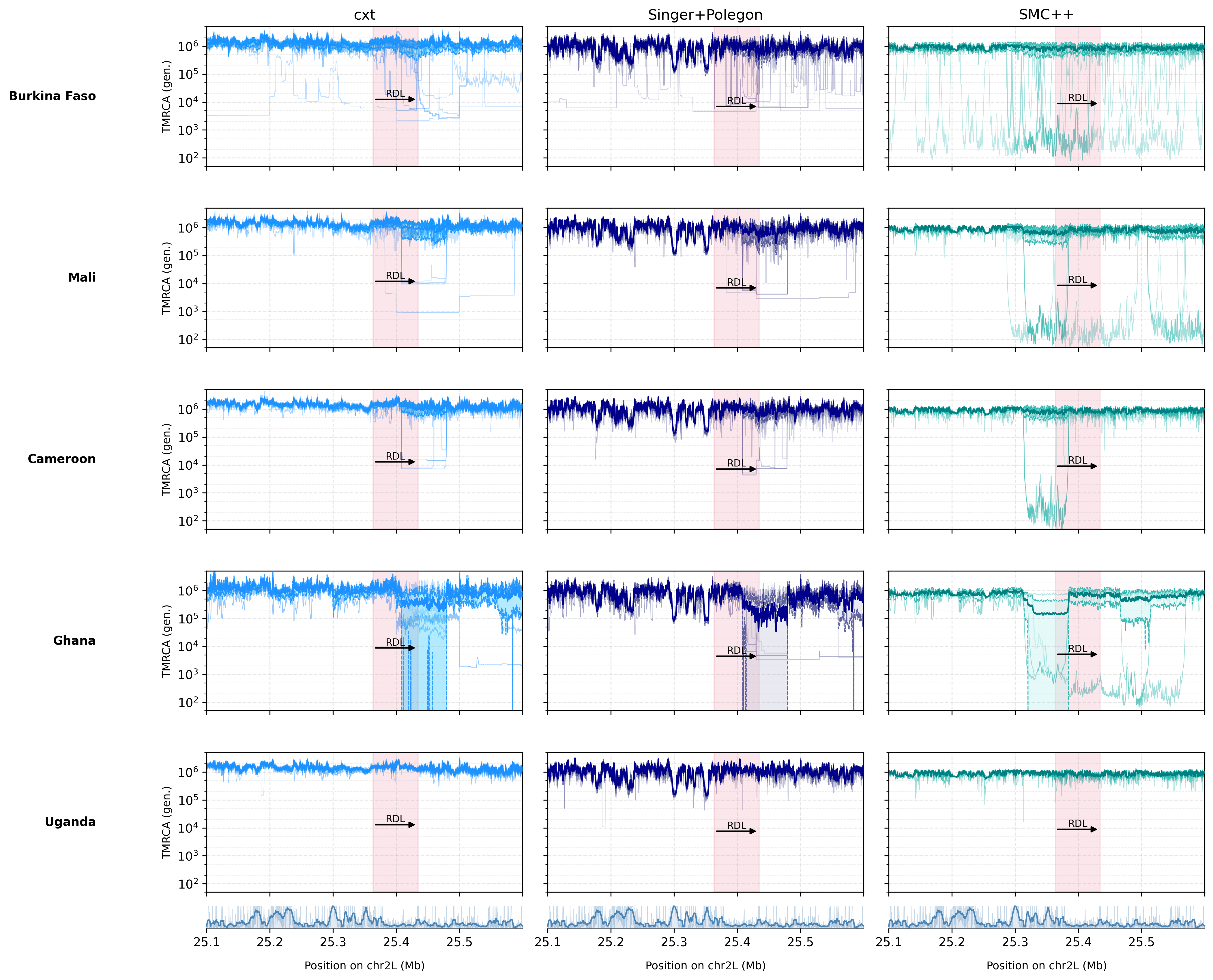
RDL region

The RDL insecticide-resistance gene spans 25.36–25.43 Mb on chr2L. The zoom window covers 25.1–25.6 Mb, showing the sharp TMRCA reduction characteristic of a selective sweep at the Rdl locus (resistance to dieldrin).

The RDL signal is visible across all five populations, with Mali and Burkina Faso showing the strongest sweep signatures, consistent with intense insecticide pressure in West Africa.

2La inversion structure

The In(2L)a inversion (approximately 20.5–42.2 Mb) creates distinct coalescent-time patterns:

• Core interval: elevated TMRCA within the inversion, reflecting reduced gene flow between karyotypes.

• Breakpoint regions: sharp TMRCA transitions at the proximal and distal inversion boundaries.

• Outside: baseline TMRCA levels in the flanking regions.

Supplementary Figure S9. Population-level comparison of TMRCA patterns across the full 2L chromosome arm.

Cross-coalescence patterns

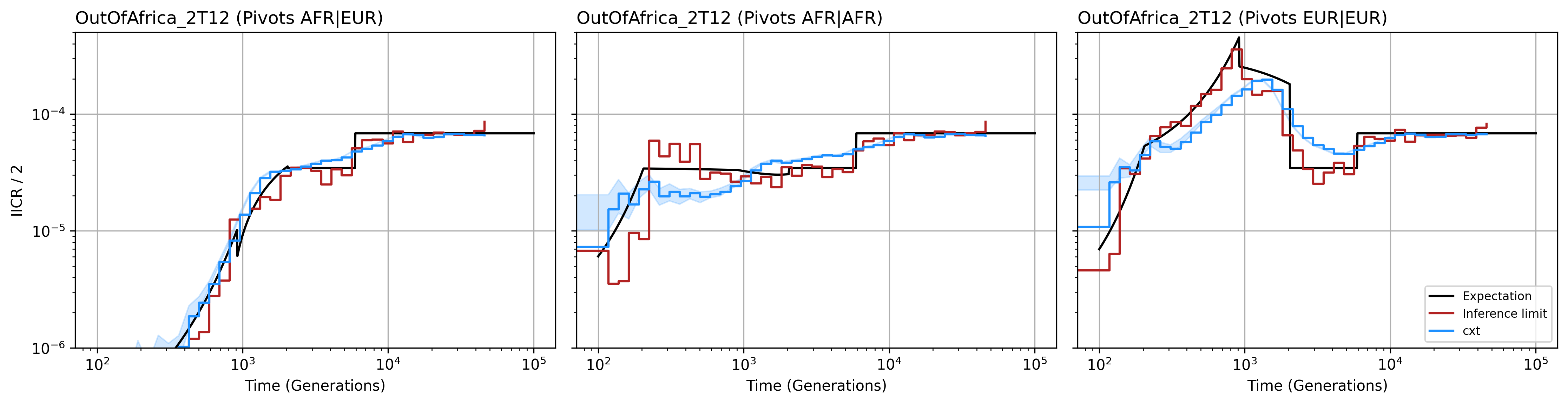
Supplementary Figure S10. Cross-coalescence patterns between populations, revealing shared and divergent demographic histories.

Reproducing the figures

The complete figure scripts with all plotting details are available at:

• figures/main/fig7_mosquito_rdl.py – RDL zoom panel (Figure 7)

• figures/main/fig8_inversion_coalescence.py – Inversion bar chart and genome-wide panels (Figure 8)

Run them via:

python figures/main/fig7_mosquito_rdl.py --output-dir figures/output/main
python figures/main/fig8_inversion_coalescence.py --output-dir figures/output/main