Examples

This page demonstrates the core cxt inference workflow: loading models, decoding pairwise TMRCA trajectories from tree sequences, and using adapter modules for sample-size transfer.

Loading pretrained models

cxt ships with seven pretrained model variants. All are loaded via cxt.load_model(), which downloads and caches checkpoints automatically.

import cxt

model_types = [
    "broad",            # main model (10 layers, w2000)
    "narrow",           # smaller model (6 layers, w2000)
    "broad_w200",       # 200 bp windows for large-Ne species
    "residual",         # log-residual targets
    "w200_wmissing",    # 200 bp windows with missingness
    "broad+adapter",    # 10-sample adapter on broad
    "w200_wmissing_adapter",  # 10-sample adapter with missingness
]

for mt in model_types:
    model = cxt.load_model(mt, device="cpu")
    n_params = sum(p.numel() for p in model.parameters())
    print(f"{mt:30s}  {n_params:>12,} parameters")

Checkpoints are cached in ~/.cache/cxt/checkpoints/ and reused on subsequent calls.

Simulating a tree sequence

For demonstration, we simulate a 1 Mb recombining tree sequence with msprime:

import msprime

ts = msprime.sim_ancestry(
    25,
    recombination_rate=1e-8,
    sequence_length=1e6,
    population_size=2e4,
    random_seed=42,
)
ts = msprime.mutate(ts, rate=1.29e-8, random_seed=42)

cxt.translate() also accepts VCF files and (genotype_matrix, positions) tuples.

Decoding pairwise TMRCA

The central inference step uses cxt.translate(). Here we decode the TMRCA trajectory for selected pivot pairs across a 1 Mb genomic block:

model = cxt.load_model("broad", device="cuda")

blocks = [(0, 1_000_000)]
pivot_pairs = [(0, 1), (2, 3), (4, 5)]
devices = ["cuda:0"]

tmrca, index_map = cxt.translate(
    ts, model,
    pivot_pairs=pivot_pairs,
    blocks=blocks,
    devices=devices,
    B=128,
    n_reps=15,
    build_workers=8,
    mutation_rate=1.29e-8,
)

Outputs:

• tmrca: log-TMRCA predictions, shape (n_items, n_reps, n_windows) when n_reps > 1, or (n_items, n_windows) otherwise.

• index_map: array of shape (n_items, 2) mapping each row to [block_idx, pivot_idx].

Key parameters:

• B: batch size per device during generation.

• n_reps: number of stochastic replicates (default 15). More replicates give smoother estimates; the mean across replicates is typically used.

• build_workers: parallel workers for SFS source construction.

• mutation_rate: if provided, applies a per-block stochastic diversity bias correction.

Multi-GPU inference

Passing multiple devices automatically shards the workload:

tmrca, index_map = cxt.translate(
    ts, model,
    pivot_pairs=pivot_pairs,
    blocks=blocks,
    devices=["cuda:0", "cuda:1", "cuda:2"],
    B_per_device=256,
    build_workers=32,
    mutation_rate=1.29e-8,
)

Sample-size transfer with adapters

Adapter models enable inference on sample sizes different from those seen during training. The broad+adapter model maps 10-sample input to the 50-sample feature space expected by the frozen backbone.

adapter_model = cxt.load_model("broad+adapter", device="cuda")

ts_n10 = ts.simplify(samples=range(10))

tmrca, index_map = cxt.translate(
    ts_n10,
    adapter_model.backbone,
    pivot_pairs=[(0, 1), (2, 3)],
    blocks=[(0, 1_000_000)],
    devices=["cuda:0"],
    B=128,
    build_workers=8,
    mutation_rate=1.29e-8,
    adapter=adapter_model.adapter,
)

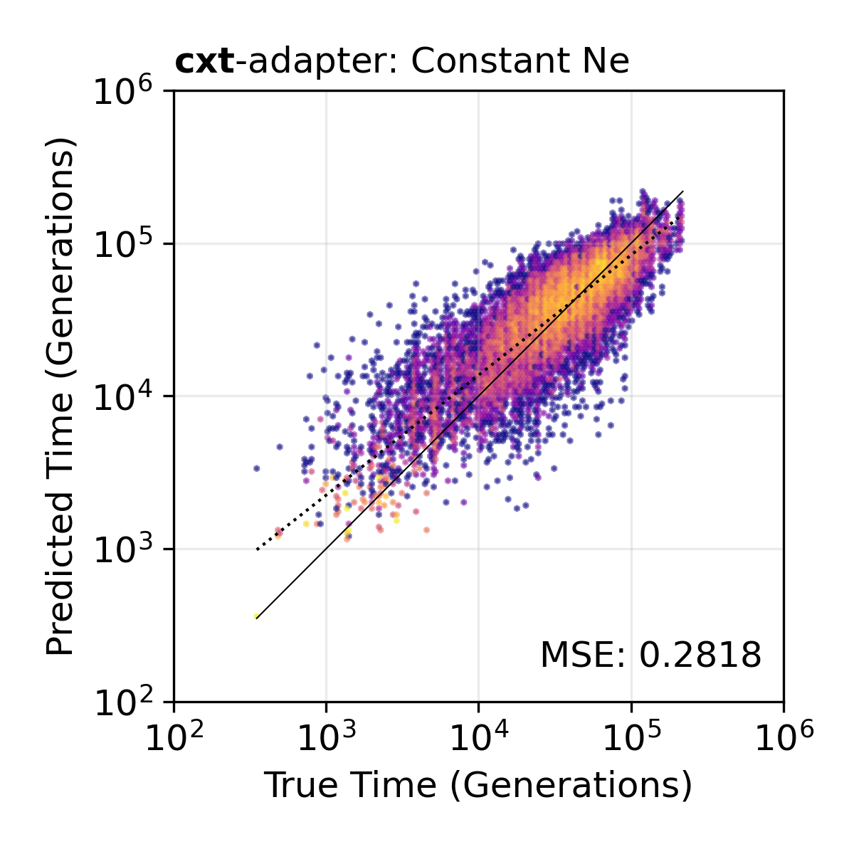
Sample-size adapter. TMRCA inference using the broad+adapter model on 10 haploid samples. The adapter learns to project 10-sample SFS features into the 50-sample space of the frozen backbone.

Window resolution variants

The broad_w200 and w200_wmissing variants use 200 bp windows instead of the default 2,000 bp, providing finer-scale resolution at the cost of a smaller effective genomic range per block. These models are especially useful for species with large effective population sizes where SFS density per window is higher.

model_w200 = cxt.load_model("broad_w200", device="cuda")

tmrca, index_map = cxt.translate(
    ts, model_w200,
    pivot_pairs=[(0, 1)],
    blocks=[(0, 100_000)],
    devices=["cuda:0"],
)

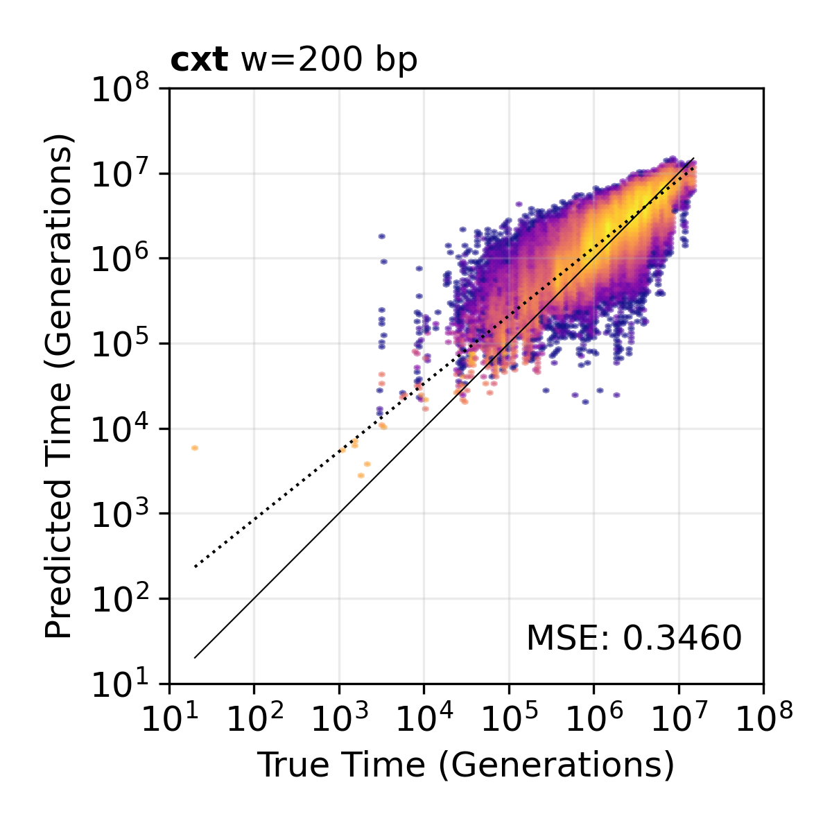
200 bp window resolution. TMRCA scatter plot at 200 bp window resolution, providing finer genomic detail.

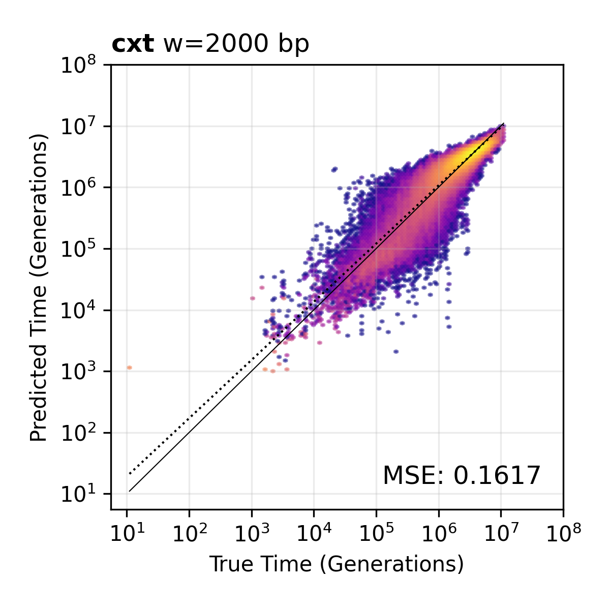
2,000 bp window resolution. The default window size used by the broad and narrow models.

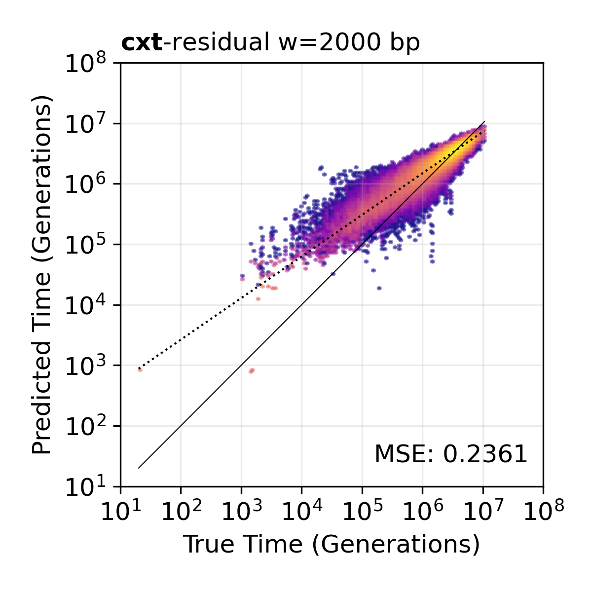
Residual model. TMRCA inference using the residual variant, which predicts log-deviations from the population mean.

Missingness-aware inference

For empirical data with missing sites (e.g. inaccessible regions in the Ag1000G), the w200_wmissing model encodes per-window missingness directly into the source tensor:

import numpy as np

model_wmissing = cxt.load_model("w200_wmissing", device="cuda")

unaccessible_bitmask = np.load("accessibility.npz")["access_2L"]
unaccessible_bitmask = ~unaccessible_bitmask

tmrca, index_map = cxt.translate(
    ts, model_wmissing,
    pivot_pairs=[(0, 1)],
    blocks=[(0, 100_000)],
    devices=["cuda:0"],
    missingness_bitmask=unaccessible_bitmask,
    mutation_rate=3.5e-9,
)

VCF input

cxt can infer TMRCAs directly from VCF files:

tmrca, index_map = cxt.translate(
    "path/to/genotypes.vcf",
    model,
    blocks=[(0, 1_000_000)],
    pivot_pairs=[(0, 1)],
    devices=["cuda:0"],
)

The VCF is parsed into a genotype matrix and positions internally using cxt.translate.vcf_parser().

Genotype matrix input

For pre-processed data, pass a (genotype_matrix, positions) tuple:

import numpy as np

gm = np.load("genotypes.npy")     # (n_haplotypes, n_sites), int
pos = np.load("positions.npy")    # (n_sites,), float, in bp

tmrca, index_map = cxt.translate(
    (gm, pos), model,
    blocks=[(0, 1_000_000)],
    pivot_pairs=[(0, 1), (2, 3)],
    devices=["cuda:0"],
)